Unsupervised Feature Selection for Time-Series Sensor Data with MSDA package

Hello, friends. In this blog post, I will take you through an use case application scenario of the algorithms with my package “msda” for the time-series sensor data. More details can be found here & refer to my previous blog post here

Here, we will see an example of unsupervised feature selection from time-series raw sensor data with my developed algorithms in the package MSDA, and further I also compare it with other well-known unsupervised techniques like PCA & IPCA.

What is MSDA?

MSDA is an open-source multidimensional multi-sensor data analysis framework, written in Python.

The variation-trend capture algorithm in MSDA module identifies events in the multidimensional time series by capturing the variation and trend to establish relationships aimed towards identifying the correlated features. With this package one can do multi-dimensional time series data analysis & supervised/unsupervised feature selection at ease. MSDA is simple, easy to use and low-code.

Why MSDA?

A simple & intuitive Python package that makes it easier to explore, plot, and visualize time-series multidimensional multi-sensor data aimed towards appropriate feature/sensor selection tasks be it the unsupervised/supervised.

Basics Revisited

Before we dwell into the usability of the package, let’s understand a few basic concepts in simple layman terms. Also, before going into deeper understanding of PCA lets first discuss a few important concepts of linear algebra.

Variance/Variation:- The variance is a measure of variability. It is calculated by taking the average of squared deviations from the mean. Variance tells you the degree of spread in your data set. The more spread in the data, the larger the variance is in relation to the mean.

Trend:- A general direction in which something is developing or changing.

Eigenvalues and Eigenvectors:- Let “A” be a n X n matrix, v is a non-zero n X 1 vector and λ is a scalar (which may be either real or complex), then any value of λ for which the below equation has a solution is known as an eigenvalue of the matrix “A”.

It is sometimes also called the characteristic value. The vector, v, which corresponds to this value is called an eigenvector

Eigenvalue Decomposition:- It is a method of splitting a matrix into a multiplication of following three matrix.

Covariance:- Covariance measures the relatedness of the two. If covariance between two variables is positive when they move in the same direction and negative otherwise. If Covariance is zero, it means the two variables are independent of each other. Covariance between two variables x and y is given by the below formula

where E[X] is the expected value of X, also known as the mean of X

Covariance Matrix:- It is a matrix whose element in the i, j position is the covariance between the i-th and j-th elements of a random vector. It is to be noted that the matrix is symmetrical and the diagonal elements of the matrix are the covariance of the variable with itself.

Principal Component Analysis:- Principal Component Analysis (PCA) is one of the most popular dimensionality reduction methods which transforms the data by projecting it to a set of orthogonal axes. It works by finding the eigenvectors and eigenvalues of the covariance matrix of the dataset. The Eigenvectors are called as the “Principal Components” of the dataset.

Incremental Principal Component Analysis:- Incremental principal component analysis (IPCA) is typically used as a replacement for principal component analysis (PCA) when the dataset to be decomposed is too large to fit in memory. IncrementalPCA only stores estimates of component and noise variances, in order update explained_variance_ratio_ incrementally. This is why memory usage depends on the number of samples per batch, rather than the number of samples to be processed in the dataset.

Multi-Sensor Data Analysis:- MSDA is a open-source, low-code time-series analysis library in Python. The fundamental principle of MSDA lies in identifying events in the multidimensional time series by capturing the variation and trend to establish relationships aimed towards finding out the most correlated features helping in feature selection process from the raw sensor signals. The algorithmic workflow in details can be found here

The features includes:-

1. Time series analysis.
2. Identifying variation of each sensor column wrt time (increasing, decreasing, equal).
3. Identifying how each column values varies wrt other column, and the maximum variation ratio between each column wrt other column.
4. Relationship establishment with trend array to identify the most appropriate sensor.
5. User can select window length and then check average value and standard deviation across each window for each sensor column.
6. It provides count of growth/decay value for each sensor column values above or below a threshold value.
7. Feature Engineering

a) Features involving trend of values across various aggregation windows: change and rate of change in average, std. deviation across window.

b) Ratio of changes, growth rate with std. deviation.

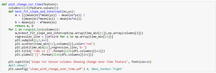
c) Change over time.

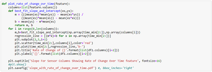
d) Rate of change over time.

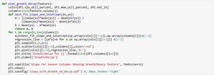
e) Growth or decay.

f) Rate of growth or decay.

g) Count of values above or below a threshold value.

EXAMPLE USECASE — Unsupervised Feature Selection

High-dimensional is very hard to process and visualize. Therefore reducing the dimensions of the data by extracting the important features (lesser than the overall number of features) which are enough to cover the variations in the data can help in the reduction of the data size and in turn for processing.

We will evaluate PCA, IPCA, and MSDA on one of Alibaba cloud virtual machine’s data (machine usage — Alibaba cluster data) containing the following attributes:-

- CPU utilization percentage (cpu_util_percent),

- memory utilization percentage (mem_util_percent),

- normalized memory bandwidth (mem_gps),

- cache miss per thousand instruction (mkpi),

- normalized incoming network traffic (net_in),

- normalized outgoing network traffic (net_out),

- disk I/O percentage (disk_io_percent).

More details about the dataset can be found here

PCA Evaluation

Steps:-

1. Import libraries

We will be using sklearn.decomposition.PCA for calculating PCA.

%matplotlib inline
import pandas as pd # for using pandas daraframe
import numpy as np # for some mathematical operations
from sklearn.preprocessing import StandardScaler # for standardizing the data
from sklearn.decomposition import PCA # for PCA calculation
import matplotlib.pyplot as plt # for plotting
import matplotlib.patches as mpatches

2. Read the data

df = pd.read_excel(‘m_1.xlsx’, index_col = 0)
df.shape

# check columns

df.columns

# peek into the data

df.head()

# The data contains “machine_id” as a column which is not required as part of # this analysis, so we have dropped it. Also, we have replaced all NaN with 0, # one could also replace them with like median or mean values.

df.drop(‘machine_id’, axis=1, inplace=True)
df = df.fillna(0)

3. Data Preprocessing

a) Standardizing the data:-

We will be using sklearn.preprocessing.StandardScaler library. It standardize the features by removing the mean and scaling to unit variance. It arranges the data in the normal distribution.

X = df.values # getting all values as matrix of dataframe
sc = StandardScaler() # creating a StandardScaler object
X_std = sc.fit_transform(X) # Standardizing the data

4. Applying PCA

An important attribute as part of it is n_components which tells the number of components to keep after applying PCA. If n_components is not set all components are kept. If n_components == 'mle' and svd_solver == 'full', Minka’s MLE is used to guess the dimension. Use of n_components == 'mle' will interpret svd_solver == 'auto' as svd_solver == 'full'.

If 0 < n_components < 1 and svd_solver == 'full', select the number of components such that the amount of variance that needs to be explained is greater than the percentage specified by n_components.

Currently, we will apply PCA without passing any parameters for the initialization of the object which means all the components are kept.

pca = PCA()
X_pca = pca.fit(X_std)

5. Determining the number of components

An important part of using PCA is to estimate how many components are needed to describe the data.

• You can get the eigenvectors using pca.components_
• eigenvalues using pca.explained_variance_
• Percentage of variance explained by each of the selected components using pca.explained_variance_ratio_

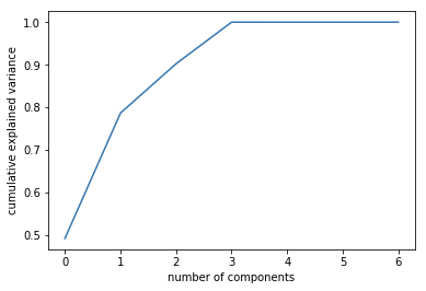
The number of components needed can be determined by looking at the cumulative explained variance ratio as a function of the number of components as shown in the below graph.

This curve quantifies how much of the total, the 7-dimensional variance is contained within the first N components. For example, we see that the first two components contain approximately 80% of the variance, while we need 4 components to describe close to 100% of the variance. Which means we can reduce our data dimension to 4 from 7 without much loss of the data.

plt.plot(np.cumsum(pca.explained_variance_ratio_))
plt.xlabel(‘number of components’)
plt.ylabel(‘cumulative explained variance’)

6. Dimensionality Reduction

Now we know that we need 4 components only, so we can apply PCA with 4 components to get the reduced dataset.

num_components = 4
pca = PCA(num_components)
X_pca = pca.fit_transform(X_std) # fit and reduce dimension

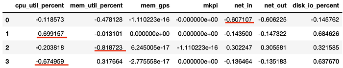
7. Finding the most important features/attribute

Now for identifying the most important feature, we have to check which features are contributing most to the components. We can see which features are contributing most to which components as shown by highlighting in the below figure (net_in, cpu_util_percent, mem_util_percent, cpu_util_percent).

pd.DataFrame(pca.components_, columns = df.columns)

8. Extracting the important features (optional)

n_pcs = pca.n_components_ # get number of component

# get the index of the most important feature on EACH component

most_important = [np.abs(pca.components_[i]).argmax() for i in
range(n_pcs)]

intial_feature_names = df.columns

# get the most important feature names

most_important_feature_names = [intial_feature_names[most_important[i]]
for i in range(n_pcs)]

most_important_feature_names

['net_in', 'cpu_util_percent', 'mem_util_percent', 'cpu_util_percent']

IPCA Evaluation

Steps:-

1. Import libraries

We will be using from sklearn.decomposition import IncrementalPCA for IPCA.

Steps 2–3 remains common

4. Applying IPCA

ipca = IncrementalPCA(n_components = 4, batch_size=10)
X_ipca = ipca.fit_transform(X_std)
print(ipca.n_components_)

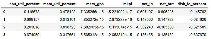
5. Finding the most important features/attribute

Now for identifying the most important feature, we have to check which features are contributing most to the components. We can see which features are contributing most to which components as shown by highlighting in the below figure (net_in, cpu_util_percent, mem_util_percent, cpu_util_percent).

pd.DataFrame(ipca.components_, columns = df.columns)

6. Extracting the important features (optional)

n_pcs_ipca = ipca.n_components_
most_important_ipca = [np.abs(ipca.components_[i]).argmax() for i in range(n_pcs_ipca)]
initial_feature_names = df.columns

#get most important feature names
most_important_feature_names_ipca = [initial_feature_names[most_important_ipca[i]]
for i in range(n_pcs_ipca)]

most_important_feature_names_ipca

['net_in', 'cpu_util_percent', 'mem_util_percent', 'cpu_util_percent']

MSDA Evaluation

Note:- Here, I am explicitly taking you through each of the available algorithms in the module without showing them being used directly from the package. For using as a package, follow the demo tutorial as shown here

Steps:-

1. Import libraries

%matplotlib inline
import pandas as pd # for using pandas daraframe
import numpy as np # for some maths operations
import matplotlib.pyplot as plt # for plotting
import matplotlib.patches as mpatches

from datetime import datetime # for creating datetime object

import operator, statistics # for calculating mean, std dev etc
from statistics import mean

2. Read the data

df1 = pd.read_excel(‘m_1.xlsx’, index_col = 0)
df1.shape

3. Extracting date & time from ‘timestamp’ column in the dataframe

df1[‘Date’] = [d.date() for d in df1.timestamp]
df1[‘Time’] = [d.time() for d in df1.timestamp]

4. Check columns

df1. columns

Index(['timestamp', 'machine_id', 'cpu_util_percent', 'mem_util_percent','mem_gps', 'mkpi', 'net_in', 'net_out', 'disk_io_percent', 'Date', 'Time'],
      dtype='object')

5. Rearrange columns, drop the unwanted fields ‘machine_id’ & the original ‘timestamp’ fields. Also, replace all NaN with 0, one could also replace them with like median or mean values.

df1 = df1[[‘timestamp’, ‘Date’, ‘Time’,’machine_id’, ‘cpu_util_percent’, ‘mem_util_percent’, ‘mem_gps’, ‘mkpi’, ‘net_in’, ‘net_out’, ‘disk_io_percent’]]

df1.drop([‘timestamp’,’machine_id’], axis=1, inplace=True)

df1 = df1.fillna(0)

6. Create a list to store logging interval of the timestamp

time_sec = []
initial=0
for i in range(len(df1.Time)):time_sec.append(initial) initial+=10

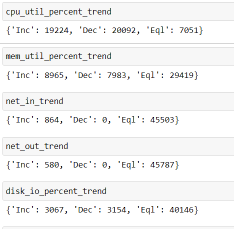
7. Identifying variation of each sensor column wrt time (increasing, decreasing, equal)

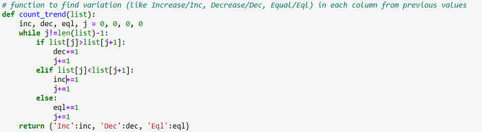
Create a list for each column & append the entries

Date, Time, cpu_util_percent, mem_util_percent, net_in, net_out, disk_io_percent = [],[],[],[],[],[],[]
Date.append(df1.Date)
Time.append(df1.Time)
cpu_util_percent.append(df1.cpu_util_percent)
mem_util_percent.append(df1.mem_util_percent)
net_in.append(df1.net_in)
net_out.append(df1.net_out)
disk_io_percent.append(df1.disk_io_percent)

# Dictionary of each column with variation
cpu_util_percent_trend = count_trend(df1.cpu_util_percent)
mem_util_percent_trend = count_trend(df1.mem_util_percent)
net_in_trend = count_trend(df1.net_in)
net_out_trend = count_trend(df1.net_out)
disk_io_percent_trend = count_trend(df1.disk_io_percent)

8. Finding maximum variation in each sensor column wrt time

# Values showing maximum variation in each column wrt Time
cpu_util_percent_trend_max = max(cpu_util_percent_trend.items(), key=operator.itemgetter(1))[0]
mem_util_percent_trend_max = max(mem_util_percent_trend.items(),key=operator.itemgetter(1))[0]
net_in_trend_max = max(net_in_trend.items(),key=operator.itemgetter(1))[0]
net_out_trend_max = max(net_out_trend.items(),key=operator.itemgetter(1))[0]
disk_io_percent_trend_max = max(disk_io_percent_trend.items(),key=operator.itemgetter(1))[0]

print(‘Max. Variation Involved in each Sensor Column values are:’)
print(‘Note: Inc-Increasing ; Dec-Decreasing ; Eq-Equal ‘)
print(‘For CPU UTIL PERCENT Column:’,cpu_util_percent_trend_max)
print(‘For MEM UTILPERCENT Column:’,mem_util_percent_trend_max)
print(‘For NET IN Column:’,net_in_trend_max)
print(‘For NET OUT Column:’,net_out_trend_max)
print(‘For DISK IO Column:’,disk_io_percent_trend_max)

Max. Variation Involved in each Sensor Column values are:
Note: Inc-Increasing ; Dec-Decreasing ; Eq-Equal 
For CPU UTIL PERCENT Column: Dec
For MEM UTILPERCENT Column: Eql
For NET IN Column: Eql
For NET OUT Column: Eql
For DISK IO Column: Eql

9. Compute Variation-Based Array to define how each column value differs from its previous value

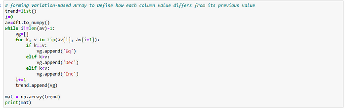
[['Eq' 'Inc' 'Dec' ... 'Eq' 'Eq' 'Eq']
 ['Eq' 'Inc' 'Inc' ... 'Eq' 'Eq' 'Eq']
 ['Eq' 'Inc' 'Inc' ... 'Eq' 'Eq' 'Eq']
 ...
 ['Eq' 'Inc' 'Dec' ... 'Eq' 'Eq' 'Eq']
 ['Eq' 'Inc' 'Dec' ... 'Eq' 'Eq' 'Inc']
 ['Eq' 'Inc' 'Inc' ... 'Eq' 'Eq' 'Eq']]

10. Find how each column value changes wrt other column values

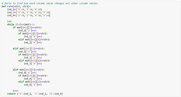
11. Calculate ratios for each variation in each column wrt other column values & finding maximum ratio to establish change of a given column wrt other column

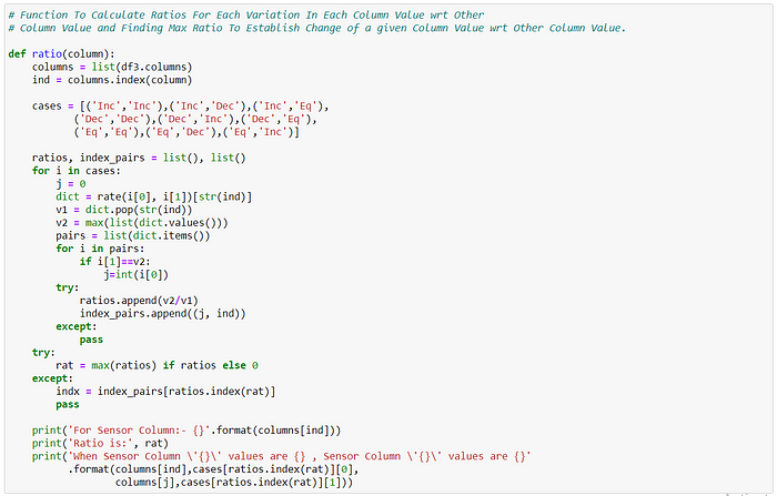
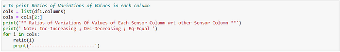
** Ratios of Variations Of Values of Each Sensor Column wrt other Sensor Column **
 Note: Inc-Increasing ; Dec-Decreasing ; Eq-Equal 
For Sensor Column:- cpu_util_percent
Ratio is: 0.6909658204509999
When Sensor Column 'cpu_util_percent' values are Eq , Sensor Column 'mem_util_percent' values are Eq
------------------------
For Sensor Column:- mem_util_percent
Ratio is: 1.0
When Sensor Column 'mem_util_percent' values are Eq , Sensor Column 'cpu_util_percent' values are Eq
------------------------
For Sensor Column:- net_in
Ratio is: 0.5092423319114361
When Sensor Column 'net_in' values are Inc , Sensor Column 'cpu_util_percent' values are Eq
------------------------

12. Detect Avg. & Std. dev across window

--------------------------------------------------------------------
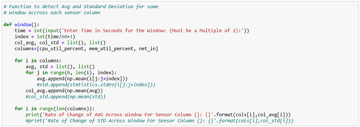
** Avg. and Standard deviations for each Sensor Column **
Enter Time in Seconds for the Window: (Must be a Multiple of 2):20
Rate of Change of AVG Across Window For Sensor Column cpu_util_percent: 34.61231884057971
Rate of Change of AVG Across Window For Sensor Column mem_util_percent: 89.74639837819186
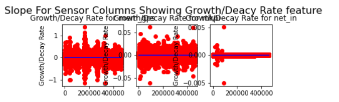
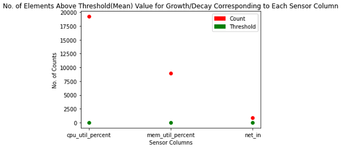
Rate of Change of AVG Across Window For Sensor Column net_in: 37.58424969806764

13. Derive new features ***: Change over time, Rate of change over time, Growth and/or decay, Rate of growth and/or decay, count of growth/decay above or below a threshold value (i.e., mean in our case).

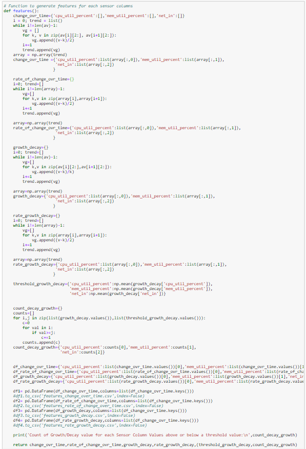
Count of Growth/Decay value for each Sensor Column Values above or below a threshold value:
 {'cpu_util_percent': 19224, 'mem_util_percent': 8965, 'net_in': 864}

14. Plot each sensor column & derived features with correlation (slope)

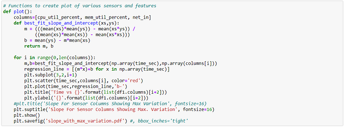
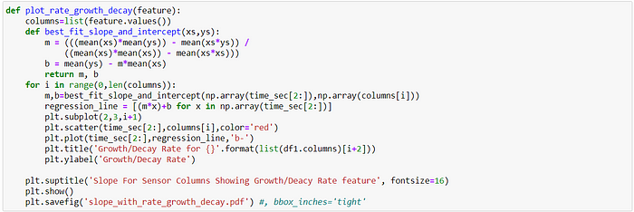
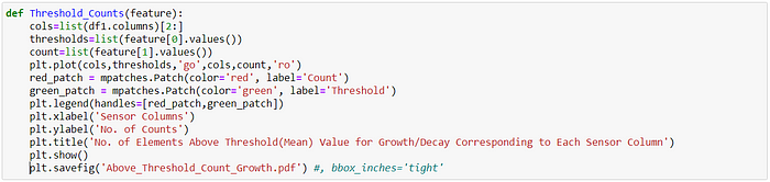
plot()

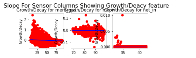
15. Based on the derived characteristics of each column, and observing the plot of characteristics & corresponding slope, we select the most appropriate column. We inspect the plots for the derived characteristics like change over time, rate of change over time, growth decay, rate growth decay, growth decay threshold counts.

MSDA Conclusion

The plots show each sensor value and features with correlation (slope) are provided.

The most appropriate sensors/features to be selected based on my variation-trend-capture-relationship approach would be then ‘net_in’, ‘mem_util_percent’ in the order of highest importance

The reasons are as follows:-

1) It has a moderate number of values above the threshold value (i.e., in our case mean).

2) The column values mostly remain constant or increase over time as seen from the slope.

3) The rate of change of column values remains constant or increases over time as seen from the slope.

4) Maximum variation within the column values shows an increasing slope.

5) It has constant decay slope.

6) Rate of Decay is positive or constant.

From my method of array values evaluation, it can be observed that the various characteristics involved in each sensor/feature column help in selection of most appropriate sensor column/features by observing the plot of the characteristics, and their corresponding slope.

Most Important Features — Comparison of PCA, IPCA, MSDA

# The top-n variables in the order of importance using the different approaches are given below.

# Top-4 features using PCA

‘net_in’, ‘cpu_util_percent’, ‘mem_util_percent’, ‘cpu_util_percent’

# Top-4 features using IPCA

‘net_in’, ‘cpu_util_percent’, ‘mem_util_percent’, ‘cpu_util_percent’

# Top features using my variation-trend-relationship-capture algorithm from the MSDA package

‘net_in’, ‘mem_util_percent’

All the code used in this blog is made available here

CONTACT

You can reach me at ajay.arunachalam08@gmail.com

Thanks for reading. Keep Learning :)